Solution using differential equation (LC circuit)
We consider the LC circuit connecting in series. We can set the differential equation. Here, both direct current (DC) and alternative current (AC) conditions are considered
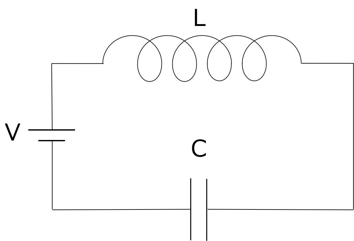
Figure 1. LC circuit for DC
Direct Current
Figure 1 shows the schematic circuit diagram of a LC circuit. The voltage of a battery is derived by the addition of voltages applied to the condenser and the coil based on Kirchhoff’s law. \begin{eqnarray} L \frac{dI}{dt} + \frac{1}{C} \int I dt = V \ \ \ \ \ \ \ \ \ \ \ \ \ \ \ (1) \end{eqnarray} where \( I \), \( L \), \( C \) are the electric current, the reactance, and capacitance of the condenser, respectively. If we differentiate Equation (1) with time, we obtain: \begin{eqnarray} L \frac{d^2 I}{dt^2} + \frac{I}{C} = 0\ \ \ \ \ \ \ \ \ \ \ \ \ \ \ (2) \end{eqnarray} As the voltage of a battery is temporary constant with time, the right-hand side of Equation (2) is zero. As you can see, the time series of the electric current of the LC circuit is expressed by the second order homogenous differential equation. By solving Equation (2), we obtain: \begin{eqnarray} I(t) = A_0 e^{- i \omega_0 t} + B_0 e^{i \omega_0 t} \ \ \ \ \ \ \ \ \ \ \ \ \ \ \ (3) \end{eqnarray} where \( \omega_0 = 1 / \sqrt{LC} \). Equation (3) can be expanded by Euler’s law: \begin{eqnarray} I(t) = A_1 \cos \omega_0 t + B_1 \sin \omega_0 t \ \ \ \ \ \ \ \ \ \ \ \ \ \ \ (4) \end{eqnarray} where \begin{align} A_1 &= A_0 + B_0 &(5) \\ B_1 &= (B_0 - A_0)i &(6) \end{align} In this way, the temporal change in the current of the LC circuit of the DC power supply can be obtained. As the LC circuit is an important circuit in electromagnetics, such as an oscillation circuit and a filter circuit which extracts a specific wavelength, you should indeed learn more deeply about this matter in an electromagnetic textbook.
Sponsored link
Alternative Current
In the case of an alternative current for the LC circuit, the differential equation for the circuit is complex. Kirchhoff’s law for a LC circuit for an alternative current is: \begin{eqnarray} L \frac{dI}{dt} + \frac{1}{C} \int I dt = V(t) \ \ \ \ \ \ \ \ \ \ \ \ \ \ \ (7) \end{eqnarray} Here, we differentiate Equation (7) with time: \begin{eqnarray} L \frac{d^2I}{dt^2} + \frac{I}{C} = \frac{d}{dt}V(t) \ \ \ \ \ \ \ \ \ \ \ \ \ \ \ (8) \end{eqnarray} This equation is an inhomogeneous second order differential equation.
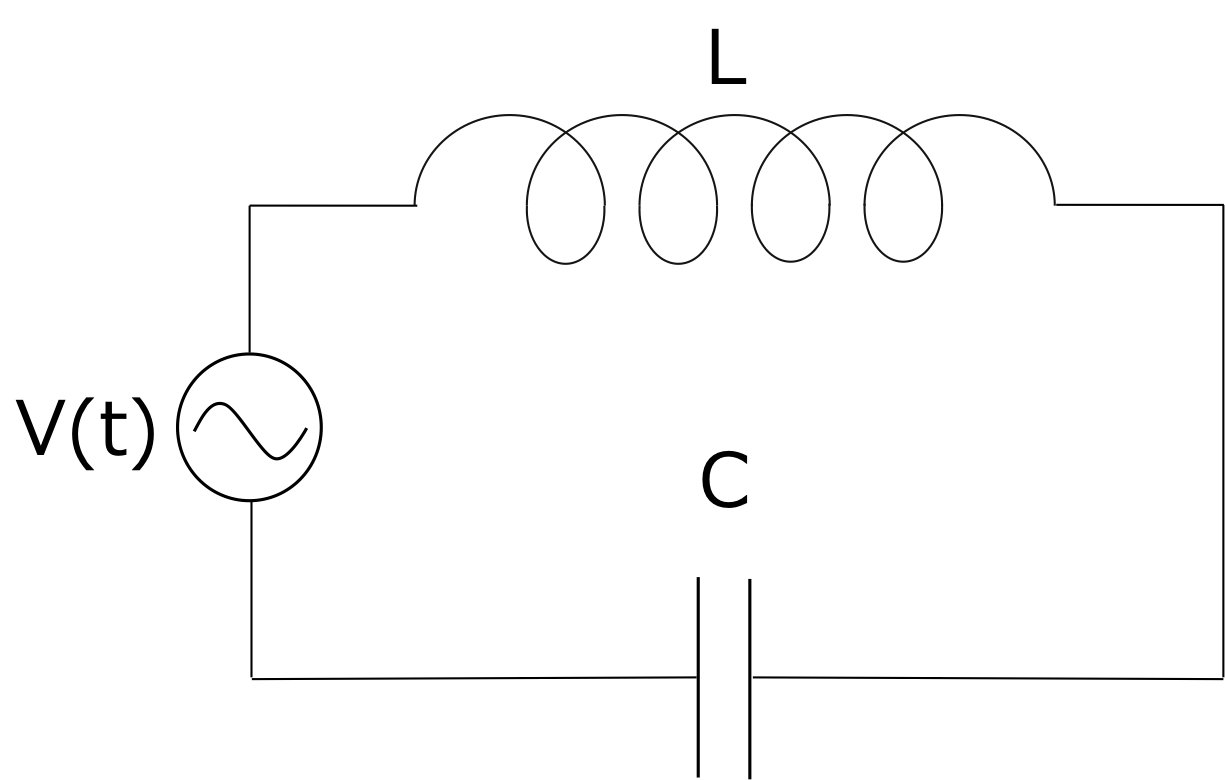
Figure 2. The LC circuit for AC.
Sponsored link