English / Japanese
Solution using differential equation (RLC circuit)

Figure 1. Schematic of an RLC circuit
Consider a circuit with a resistor \(R\), a coil \(L\), and a capacitor \(C\) connected as shown in Figure 1.
This circuit is called an RLC circuit.
The RLC circuit is important in an AC power supply to study electromagnetism, but here we only consider the case of a DC power supply.
When the RLC circuit is connected to a DC power supply with an applied voltage \(V\), we can define the equation using Kirchhoff's law:
\begin{eqnarray}
RI + L \frac{dI}{dt} + \frac{1}{C}\int I dt = V\ \ \ \ \ \ \ \ \ \ \ \ \ \ \ \ \ \ \ \ (1)
\end{eqnarray}
where I is the electric current, \( L \) is the reactance, and \( C \) is the capacitance.
We differentiate Equation (1) in time as follow:
\begin{eqnarray}
R \frac{dI}{dt} + L \frac{d^2I}{dt^2} + \frac{I}{C} = 0\ \ \ \ \ \ \ \ \ \ \ \ \ \ \ \ \ \ \ \ (2)
\end{eqnarray}
If we assume the solution would be expressed by \( e^{\lambda t} \), the characteristic equation becomes:
\begin{eqnarray}
L \lambda^2 + R \lambda + \frac{1}{C} = 0\ \ \ \ \ \ \ \ \ \ \ \ \ \ \ \ \ \ \ \ (3-1)
\end{eqnarray}
Equation (3-1) is written as follows:
\begin{eqnarray}
\lambda^2 + \frac{R}{L} \lambda + \frac{1}{LC} = 0\ \ \ \ \ \ \ \ \ \ \ \ \ \ \ \ \ \ \ \ (3-2)
\end{eqnarray}
By solving the above Equation (3-2), \( \lambda \) becomes:
\begin{eqnarray}
\lambda = - \frac{R}{2L} \pm \sqrt{ \left( \frac{R}{2L} \right)^2 - \frac{1}{LC} } \ \ \ \ \ \ \ \ \ \ \ \ \ \ \ \ \ \ \ \ (4)
\end{eqnarray}
Thus, the electric current \( I(t) \) is:
\begin{eqnarray}
I(t) &=& Ae^{ \left( - \frac{R}{2L} + \sqrt{ \left( \frac{R}{2L} \right)^2 - \frac{1}{LC} } \right) t } +
Be^{ \left( - \frac{R}{2L} - \sqrt{ \left( \frac{R}{2L} \right)^2 - \frac{1}{LC} } \right) t } \\
&=& e^{ - \frac{R}{2L} t } \left\{ Ae^{ \left( \sqrt{ \left( \frac{R}{2L} \right)^2 - \frac{1}{LC} } \right) t}
+ Be^{ \left(- \sqrt{ \left( \frac{R}{2L} \right)^2 - \frac{1}{LC} } \right) t} \right\} \ \ \ \ \ \ \ \ \ \ \ \ \ \ \ \ \ \ \ \ (5)
\end{eqnarray}
This equation is similar to the equation for the damped oscillation.
Hence, depending on \((R/2L)^2\) being larger or equal to \(1/LC\), the time series of current.
Below, I intend to explain this using Figure 2, representing the current change with time.
Sponsored link
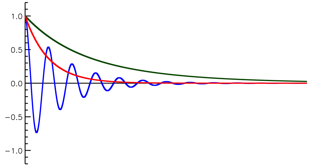
Figure 2. The time series of the electric current represented as overdamped (green), damped oscillation (blue), and critical damping (red).
\( \left( R/2L \right)^2 > 1/LC \)
In this case, \( \sqrt{ \left( \frac{R}{2L} \right)^2 - \frac{1}{LC} } \) is real.
Thus, the electric current will exponentially decay with time.
This decay is called overdamped.
\( \left( R/2L \right)^2 < 1/LC \)
In this case, the shoulder of e is imaginary. Using Euler’s formula, Equation 5 is expressed as follows:
\begin{eqnarray}
I(t) = e^{ - \frac{R}{2L} t } \left( C_1 \cos \sqrt{ \left( \frac{1}{LC} - \frac{R}{2L} \right)^2 } t
+ C_2 \sin \sqrt{ \left( \frac{1}{LC} - \frac{R}{2L} \right)^2 } t \right)
\end{eqnarray}
where \(C_1\) and \(C_2\) are constant.
As you can see in this equation, the electric current oscillates with the decay.
The oscillation of the electric current is shown in Figure 2. The decay rate is:
\begin{eqnarray}
e^{ - \frac{R}{2L} t }
\end{eqnarray}
This decay is called the damped oscillation.
\( \left( R/2L \right)^2 = 1/LC \)
In this case, the shoulder of \(e\) is zero. The electric current can be expressed as:
\begin{eqnarray}
I(t) = e^{ - \frac{R}{2L} t } (A + Bt)
\end{eqnarray}
The electric current defined by the above equation is the fastest decay, as shown by the red line in Figure 2.
This decay is called the critical damping.
Sponsored link