English / Japanese
Solution using differential equation (Damped oscillation)
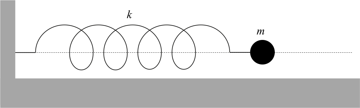
Figure 1. The material point connecting with the spring.
As shown in Figure 1, we consider the material point connecting with the spring.
In general, the frictions between the material and the floor re neglected.
However, in this page, we consider the situation with frictions being proportional to the velocity of the material \(v=dx/dt\).
The momentum equation for this material point is:
\begin{eqnarray}
m \frac{d^2x}{dt^2} = - kx - b\frac{dx}{dt}\ \ \ \ \ \ \ \ \ \ \ \ \ \ (1)
\end{eqnarray}
where m is the mass of this material point, k is the spring-constant, and b is the factor of proportionality for the frictional force.
Equation (1) is the homogeneous differential equation. We modify Equation (1) as follows:
\begin{eqnarray}
\frac{d^2 x}{dt^2} + \frac{b}{m} \frac{dx}{dt} + \frac{k}{m} x = 0\ \ \ \ \ \ \ \ \ \ \ \ \ \ (2)
\end{eqnarray}
If we assume that the solution for Equation (2) becomes of the form of \(e^{\lambda t}\), the characteristic equation for Equation (2) becomes:
\begin{eqnarray}
\lambda^2 + \frac{b}{m} \lambda + \frac{k}{m} = 0\ \ \ \ \ \ \ \ \ \ \ \ \ \ (3)
\end{eqnarray}
We define:
\begin{eqnarray}
\gamma &=& \frac{b}{2m} \\
\omega &=& \sqrt{ \frac{k}{m} }
\end{eqnarray}
If we substitute the above constants to the characteristic equation, we obtain:
\begin{eqnarray}
\lambda^2 + 2 \gamma \lambda + \omega^2 = 0\ \ \ \ \ \ \ \ \ \ \ \ \ \ (4)
\end{eqnarray}
This equation can be easily solved as follows:
\begin{eqnarray}
\lambda = - \gamma \pm \sqrt{\gamma^2 - \omega^2}\ \ \ \ \ \ \ \ \ \ \ \ \ \ (5)
\end{eqnarray}
Thus, the solution of Equation (2) is:
\begin{eqnarray}
x &=& A e^{ \left(- \gamma + \sqrt{\gamma^2 - \omega^2} \right)t } + B e^{ \left(- \gamma - \sqrt{\gamma^2 - \omega^2} \right)t } \\
&=& e^{-\gamma t} \left\{ A e^{\sqrt{\gamma^2 - \omega^2}t} + Be^{-\sqrt{\gamma^2 - \omega^2}t} \right\}\ \ \ \ \ \ \ \ \ \ \ \ \ \ (6)
\end{eqnarray}
where \(A\) and \(B\) are constants.
Thus, the forced oscillation depends on \( \gamma^2 - \omega^2 \) being positive, negative, or equal.
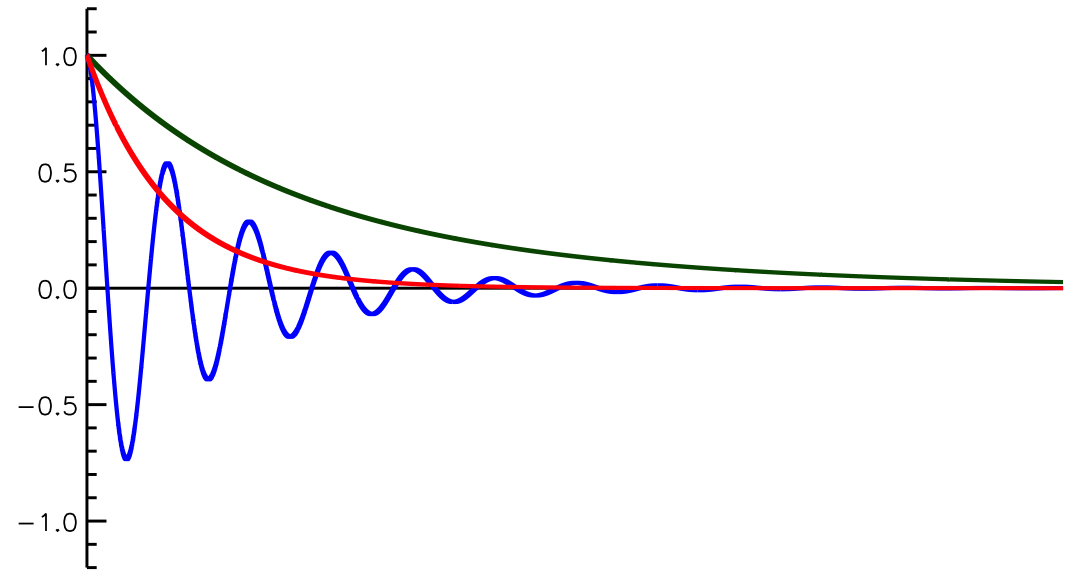
Figure 2. The time series of the material point. The green, blue, and red lines show the overdamping, damped oscillation, and critical damping, respectively.
\( \gamma > \omega \)
In this case, \(\sqrt{\gamma^2-\omega^2 }\) becomes real.
Hence, \(x\) converges with the time scale of \(e^{-\gamma t}\), as illustrated by the green line in Figure 2.
The material point does not oscillate in this case.
This damped oscillation is called overdamping.
\( \gamma < \omega \)
In this case, \( \sqrt{\gamma^2- \omega^2 } \) becomes imaginary and Equation (6) can be expanded with the trigonometric function using the Euler’s formula, as follows:
\begin{eqnarray}
x = e^{-\gamma t} \left( C_1 \cos \sqrt{\omega^2 - \gamma^2}t + C_2 \sin \sqrt{\omega^2 - \gamma^2}t \right)\ \ \ \ \ \ \ \ \ \ \ \ \ \ (7)
\end{eqnarray}
where \(C_1\) and \(C_2\) are constants.
We simplify Equation (7) using trigonometric functions:
\begin{eqnarray}
x = e^{-\gamma t} C_0 \sin \left( \sqrt{\omega^2 - \gamma^2}t + \phi \right)\ \ \ \ \ \ \ \ \ \ \ \ \ \ (8)
\end{eqnarray}
where \(C_0=\sqrt{C_1^2+C_2^2}\) and \( \tan \phi =C_2/C_1\).
The material point oscillates with the damped function of \(e^{-\gamma t}\) and converges to \(x=0\).
This oscillation is damped oscillation.
\( \gamma = \omega \)
If \(\gamma\) and \(\omega\) are equal, Equation (6) simply becomes:
\begin{eqnarray}
x = e^{-\gamma t} (A+Bt)\ \ \ \ \ \ \ \ \ \ \ \ \ \ (9)
\end{eqnarray}
In this case, the material point damped most rapidly, as illustrated by the red line in Figure 2.
This damped oscillation is called the critical damping.
Sponsored link